This tutorial walks you through a complete risk assessment using the ecorisk package with provided demo datasets. For background on the underlying framework and theory, see the Background & Framework article.
Scenario
Let’s suppose we want to conduct a risk assessment for a fictional marine ecosystem. We want to investigate whether the system is at risk of being in an undesired state due to 5 ongoing pressures:
- Temperature increase due to climate change
- Salinity decrease due to climate change
- A decreasing nutrient input after a phase of eutrophication
- Oxygen depletion
- Fishing pressure
To best represent our ecosystem we choose state indicators from different trophic levels: phytoplankton, zooplankton, two fish species (herring and cod), and seabirds. For some of these we have more or less detailed expert knowledge and for some of them we have time series representing this state indicator. Thus we decide on the following assessment scheme using both the expert scoring and the modelling pathway of ecorisk:
| Trait | General | Model |
|---|---|---|
| Cod | Phytoplankton | Cod spawning stock biomass |
| Herring | Seabirds | Zooplankton mean size |
For the two fish species enough knowledge is available for a detailed expert scoring using species traits. Phytoplankton and seabirds are larger species groups, a scoring on a trait basis would be very difficult, therefore the experts will give here only one general score for sensitivity and adaptive capacity of these two groups. The time series we want to use for the modeling approach are i) spawning stock biomass of the cod stock as indicator for the health of the species and ii) zooplankton mean size which represents the status of the zooplankton group and gives an indication about the status of the food web. The pressures will be assessed using both pathways.
Data preparation
First step is to create the scoring tables, which will be filled out
by our experts. With the functions
create_template_exposure() and
crt_sensitivity(), we can automatically create tables for
further usage in the ecorisk workflow. The functions need the names of
the pressures and for sensitivity also the names of the indicators. For
exposure we want to investigate 4 components:
The magnitude of change,
the future trend,
the frequency of the change and
the spatial coverage of the change in the ecosystem.
To define vulnerability the experts should score the sensitivity and the adaptive capacity. They should differentiate between two types of effect: direct effects only and the combination of direct and indirect effects. Indirect effects occur for example due to food web interactions. If possible the experts will score four individual species traits:
Feeding
Behaviour
Reproduction
Habitat
otherwise they will give general sensitivity and adaptive capacity scores. Both the exposure and the sensitivity scoring include an uncertainty assessment. As a second step we rename the variables in our scoring templates.
exposure_scoring <- create_template_exposure(
  pressures = c("temperature", "salinity", "oxygen", "nutrient", "fishing"),
  n_components = 4,
  mode_uncertainty = "component"
)
names(exposure_scoring)
#> [1] "pressure"                "component_1"
#> [3] "component_2"             "component_3"
#> [5] "component_4"             "uncertainty_component_1"
#> [7] "uncertainty_component_2" "uncertainty_component_3"
#> [9] "uncertainty_component_4"
# Rename exposure components
names(exposure_scoring)[2:9] <- c("magnitude", "frequency", "trend", "spatial",
                                  "uncertainty_magnitude", "uncertainty_frequency",
                                  "uncertainty_trend", "uncertainty_spatial")

sensitivity_scoring <- create_template_sensitivity(
  indicators = c("phytoplankton", "herring", "cod", "seabirds"),
  pressures = c("temperature", "salinity", "oxygen", "nutrient", "fishing"),
  type = c("direct", "direct_indirect"),
  n_sensitivity_traits = 5,
  mode_adaptive_capacity = "trait",
  mode_uncertainty = "trait"
)
names(sensitivity_scoring)
#>  [1] "indicator"                "pressure"
#>  [3] "type"                     "sens_trait_1"
#>  [5] "sens_trait_2"             "sens_trait_3"
#>  [7] "sens_trait_4"             "sens_trait_5"
#>  [9] "ac_trait_1"               "ac_trait_2"
#> [11] "ac_trait_3"               "ac_trait_4"
#> [13] "ac_trait_5"               "uncertainty_sens_trait_1"
#> [15] "uncertainty_sens_trait_2" "uncertainty_sens_trait_3"
#> [17] "uncertainty_sens_trait_4" "uncertainty_sens_trait_5"
#> [19] "uncertainty_ac_trait_1"   "uncertainty_ac_trait_2"
#> [21] "uncertainty_ac_trait_3"   "uncertainty_ac_trait_4"
#> [23] "uncertainty_ac_trait_5"

# Replace the generic trait names ('...trait_1', '...trait_2') with
# the actual trait names
names(sensitivity_scoring) <- names(sensitivity_scoring) |>
  stringr::str_replace("trait_1$", "feeding") |>
  stringr::str_replace("trait_2$", "behaviour") |>
  stringr::str_replace("trait_3$", "reproduction") |>
  stringr::str_replace("trait_4$", "habitat") |>
  stringr::str_replace("trait_5$", "general")
The experts have filled out the scoring tables in a joint exercise, thus we do not have to aggregate the individual expert scores. If individual expert scores are given, it is recommended to follow the work flow until the risk calculation and aggregation of risk scores is completed and then aggregate these scores across all experts. This allows for more precise and detailed results, as differences in the results between experts can be evaluated.
exposure_scoring <- ex_expert_exposure
head(exposure_scoring)
#>      pressure magnitude frequency trend spatial uncertainty_magnitude
#> 1 temperature         1         1     4       5                     1
#> 2    salinity         1         4     1       3                     2
#> 3      oxygen         1         1     1       2                     2
#> 4    nutrient         2         2     3       2                     1
#> 5     fishing         5         4     5       2                     3
#>   uncertainty_frequency uncertainty_trend uncertainty_spatial
#> 1                     1                 3                   3
#> 2                     2                 2                   2
#> 3                     2                 3                   3
#> 4                     2                 2                   3
#> 5                     1                 2                   1
sensitivity_scoring <- ex_expert_sensitivity
head(sensitivity_scoring)
#>       indicator    pressure            type sens_feeding sens_behaviour
#> 1 phytoplankton temperature          direct           NA             NA
#> 2 phytoplankton    salinity          direct           NA             NA
#> 3 phytoplankton      oxygen          direct           NA             NA
#> 4 phytoplankton    nutrient          direct           NA             NA
#> 5 phytoplankton     fishing          direct           NA             NA
#> 6 phytoplankton temperature direct_indirect           NA             NA
#>   sens_reproduction sens_habitat sens_general ac_feeding ac_behaviour
#> 1                NA           NA           -3         NA           NA
#> 2                NA           NA            0         NA           NA
#> 3                NA           NA           -2         NA           NA
#> 4                NA           NA           -3         NA           NA
#> 5                NA           NA            0         NA           NA
#> 6                NA           NA           -4         NA           NA
#>   ac_reproduction ac_habitat ac_general uncertainty_sens_feeding
#> 1              NA         NA          1                       NA
#> 2              NA         NA          1                       NA
#> 3              NA         NA          1                       NA
#> 4              NA         NA          1                       NA
#> 5              NA         NA          0                       NA
#> 6              NA         NA          1                       NA
#>   uncertainty_sens_behaviour uncertainty_sens_reproduction
#> 1                         NA                            NA
#> 2                         NA                            NA
#> 3                         NA                            NA
#> 4                         NA                            NA
#> 5                         NA                            NA
#> 6                         NA                            NA
#>   uncertainty_sens_habitat uncertainty_sens_general uncertainty_ac_feeding
#> 1                       NA                        1                     NA
#> 2                       NA                        2                     NA
#> 3                       NA                        2                     NA
#> 4                       NA                        2                     NA
#> 5                       NA                        1                     NA
#> 6                       NA                        1                     NA
#>   uncertainty_ac_behaviour uncertainty_ac_reproduction uncertainty_ac_habitat
#> 1                       NA                          NA                     NA
#> 2                       NA                          NA                     NA
#> 3                       NA                          NA                     NA
#> 4                       NA                          NA                     NA
#> 5                       NA                          NA                     NA
#> 6                       NA                          NA                     NA
#>   uncertainty_ac_general
#> 1                      1
#> 2                      2
#> 3                      2
#> 4                      2
#> 5                      1
#> 6                      1
The experts followed this scoring scheme:
Exposure 1–5 (low to high)
Sensitivity −5–5 (high negative to high positive influence)
Adaptive capacity −1–1 (low to high)
Uncertainty 1–3 (low to high)
For more information about this scheme see also the Scoring section in the Background article. This scoring scheme aligns with the results of the modelling pathway.
To prepare the modelling pathway we load our time series data. The data includes indicator variables for our five pressures and two state indicators (cod and zooplankton). The data covers a time frame from 1984 to 2016. The data was created based on trends of similar indicators from the Baltic Sea. There is another example data set with data from the North Sea.
ts_pressures <- pressure_ts_baltic
head(ts_pressures)
#>   year nitrogen phosphorous surf_temp_sum bot_temp_ann surf_sal_sum bot_sal_ann
#> 1 1984 20.75630   0.5909141      14.64714     4.626137     6.177466    8.831664
#> 2 1985 20.69365   0.5167932      12.24114     4.049684     6.206347    8.715647
#> 3 1986 21.00117   0.5564102      12.24247     4.047897     6.228291    8.144442
#> 4 1987 21.12562   0.4828138      10.25126     3.915981     5.984160    8.349860
#> 5 1988 19.33260   0.5308540      13.96107     4.418284     5.909042    8.166351
#> 6 1989 20.88782   0.5963618      13.65516     4.942516     5.875959    7.925876
#>   bot_oxy_ann fishing_cod
#> 1    4.298515   0.7798201
#> 2    4.325501   0.7705255
#> 3    4.598441   0.9276049
#> 4    4.310448   0.8718370
#> 5    4.096484   0.8253639
#> 6    4.248611   0.9619950
ts_indicators <- indicator_ts_baltic
head(ts_indicators)
#>   year zooplankton_mean_size eastern_baltic_cod
#> 1 1984              24.46262           662.0919
#> 2 1985              11.72344           548.5772
#> 3 1986              13.71266           402.0580
#> 4 1987              15.14893           322.6262
#> 5 1988              24.91170           301.2875
#> 6 1989              11.86890           241.8906
Analysis
Now we will calculate exposure and sensitivity scores in both
pathways. We start with the expert scoring pathway using the functions
calc_exposure() and calc_sensitivity(). They
calculate from the exposure components and sensitivity trait scores
general scores using an aggregation method selected by the user. We will
use the arithmetic mean to aggregate component and trait scores. Other
options are median, minimum or maximum.
exp_expert <- calc_exposure(
  pressures = exposure_scoring$pressure,
  components = exposure_scoring[ ,2:5],
  uncertainty = exposure_scoring[ ,6:9],
  method = "mean"
)
head(exp_expert)
#>      pressure exposure uncertainty
#> 1 temperature     2.75        2.00
#> 2    salinity     2.25        2.00
#> 3      oxygen     1.25        2.50
#> 4    nutrient     2.25        2.00
#> 5     fishing     4.00        1.75

sens_ac_expert <- calc_sensitivity(
  indicators = sensitivity_scoring$indicator,
  pressures = sensitivity_scoring$pressure,
  type = sensitivity_scoring$type,
  sensitivity_traits = sensitivity_scoring[ ,4:8],
  adaptive_capacities = sensitivity_scoring[ ,9:13],
  uncertainty_sens = sensitivity_scoring[ ,14:18],
  uncertainty_ac = sensitivity_scoring[ ,19:23],
  method = "mean"
)
head(sens_ac_expert)
#>       indicator    pressure            type pathway sensitivity
#> 1 phytoplankton temperature          direct  expert          -3
#> 2 phytoplankton    salinity          direct  expert           0
#> 3 phytoplankton      oxygen          direct  expert          -2
#> 4 phytoplankton    nutrient          direct  expert          -3
#> 5 phytoplankton     fishing          direct  expert           0
#> 6 phytoplankton temperature direct_indirect  expert          -4
#>   adaptive_capacity uncertainty_sens uncertainty_ac sens_original.sens_feeding
#> 1                 1                1              1                         NA
#> 2                 1                2              2                         NA
#> 3                 1                2              2                         NA
#> 4                 1                2              2                         NA
#> 5                 0                1              1                         NA
#> 6                 1                1              1                         NA
#>   sens_original.sens_behaviour sens_original.sens_reproduction
#> 1                           NA                              NA
#> 2                           NA                              NA
#> 3                           NA                              NA
#> 4                           NA                              NA
#> 5                           NA                              NA
#> 6                           NA                              NA
#>   sens_original.sens_habitat sens_original.sens_general ac_original.ac_feeding
#> 1                         NA                         -3                     NA
#> 2                         NA                          0                     NA
#> 3                         NA                         -2                     NA
#> 4                         NA                         -3                     NA
#> 5                         NA                          0                     NA
#> 6                         NA                         -4                     NA
#>   ac_original.ac_behaviour ac_original.ac_reproduction ac_original.ac_habitat
#> 1                       NA                          NA                     NA
#> 2                       NA                          NA                     NA
#> 3                       NA                          NA                     NA
#> 4                       NA                          NA                     NA
#> 5                       NA                          NA                     NA
#> 6                       NA                          NA                     NA
#>   ac_original.ac_general
#> 1                      1
#> 2                      1
#> 3                      1
#> 4                      1
#> 5                      0
#> 6                      1
Both data sets now contain the aggregated expert scores. The sensitivity dataset also contains the initial expert scores, thus we can still calculate vulnerability for each trait individually, which will lead to more precise results. Additionally the last column gives information about the pathway of the scores to compare later on the results from both pathways.
In the modelling pathway we use the functions
model_exposure() and model_sensitivity(). To
assess exposure based on a time series we have to define a period where
baseline conditions are assumed, the baseline conditions are then
compared to the conditions in the assessment time period. In this
tutorial the baseline is set to the first 10 years of the time series
and the assessment time period are the last 5 years of the time series.
Since baseline conditions are considered as “good” for our ecosystem all
pressures should return to baseline conditions, we specify this with the
argument trend. The spatial scale cannot be assessed with temporal data
only, thus we have to specify the scores. We use here the same value for
the spatial component that the experts gave for the pressures in the
expert scoring.
exposure_model <- model_exposure(
  pressure_time_series = ts_pressures,
  base_years = c(start = 1984, end = 1993),
  current_years = c(start = 2007, end = 2016),
  trend = "return",
  spatial = c(2, 2, 5, 5, 3, 3, 2, 2)
)
exposure_model
#>        pressure exposure uncertainty comp_magnitude comp_frequency comp_trend
#> 1      nitrogen     3.25           2              3              5          3
#> 2   phosphorous     2.00           2              1              2          3
#> 3 surf_temp_sum     3.25           2              2              3          3
#> 4  bot_temp_ann     3.50           2              2              4          3
#> 5  surf_sal_sum     3.25           2              2              5          3
#> 6   bot_sal_ann     2.75           3              1              3          4
#> 7   bot_oxy_ann     3.00           2              2              5          3
#> 8   fishing_cod     3.25           3              3              5          3
#>   comp_direction comp_spatial uncertainty_arima uncertainty_gam mean_baseline
#> 1       increase            2                 2               3    19.8141436
#> 2       increase            2                 2               2     0.5734645
#> 3       increase            5                 2               2    13.2227690
#> 4       increase            5                 2               2     4.7876146
#> 5       decrease            3                 2               2     5.9609406
#> 6       decrease            3                 3               3     8.2235847
#> 7       decrease            2                 2               2     4.4527522
#> 8       decrease            2                 3               3     0.8957243
#>   mean_current standard_deviation_baseline slope_linear_model
#> 1   22.4085515                  1.27462524         0.13135681
#> 2    0.6287693                  0.07808664         0.15626299
#> 3   14.7021123                  1.33356555         0.20863265
#> 4    6.1324167                  0.72058273         0.02144553
#> 5    5.6123374                  0.18378270        -0.12287663
#> 6    7.9426842                  0.33153236        -0.30833474
#> 7    4.0093738                  0.26302107        -0.15798683
#> 8    0.4765706                  0.20083878        -0.13339762
#>   p_value_linear_model
#> 1         2.550606e-01
#> 2         1.672706e-01
#> 3         5.010921e-02
#> 4         8.585639e-01
#> 5         2.897796e-01
#> 6         7.878018e-05
#> 7         1.619831e-01
#> 8         2.470676e-01
The output gives us the aggregated exposure score, which is the
arithmetic mean of all exposure components. These are the same
components that have been evaluated by our experts. The
model_exposure() function does not evaluate the associated
uncertainty.
We should check for all pressures if the direction is capturing the correct dynamics and not only a short term fluctuation.
To assess sensitivity with time series data we also have to specify the assessment time period to determine if the pressure has in the assessment time period a negative or positive influence on the state indicator. The influence is determined using a simple linear model, so we can simply check if the direction was correctly determined using a simple plot. First we set up a data frame specifying for each indicator pressure combination the assessment time period.
sens_ac_model <- model_sensitivity(
  indicator_time_series = ts_indicators,
  pressure_time_series = ts_pressures,
  current_years = c(start = 2010, end = 2016)
)
#> Please review the model diagnostics of the GAMs applied in the time series based sensitivity scoring using the function plot_diagnostic_sensitivity(). Remove models with unacceptable diagnostics from the output table of this function.
sens_ac_model
#>                indicator      pressure            type pathway sensitivity
#> 1  zooplankton_mean_size      nitrogen direct_indirect   model           3
#> 2  zooplankton_mean_size   phosphorous direct_indirect   model           0
#> 3  zooplankton_mean_size surf_temp_sum direct_indirect   model           0
#> 4  zooplankton_mean_size  bot_temp_ann direct_indirect   model           0
#> 5  zooplankton_mean_size  surf_sal_sum direct_indirect   model          -1
#> 6  zooplankton_mean_size   bot_sal_ann direct_indirect   model          -1
#> 7  zooplankton_mean_size   bot_oxy_ann direct_indirect   model           0
#> 8  zooplankton_mean_size   fishing_cod direct_indirect   model           0
#> 9     eastern_baltic_cod      nitrogen direct_indirect   model          -1
#> 10    eastern_baltic_cod   phosphorous direct_indirect   model           0
#> 11    eastern_baltic_cod surf_temp_sum direct_indirect   model          -1
#> 12    eastern_baltic_cod  bot_temp_ann direct_indirect   model          -3
#> 13    eastern_baltic_cod  surf_sal_sum direct_indirect   model           3
#> 14    eastern_baltic_cod   bot_sal_ann direct_indirect   model           0
#> 15    eastern_baltic_cod   bot_oxy_ann direct_indirect   model           1
#> 16    eastern_baltic_cod   fishing_cod direct_indirect   model          -1
#>    adaptive_capacity uncertainty_sens uncertainty_ac          r_sq      p_value
#> 1                  0                2             NA  0.2431778963 0.0172601903
#> 2                  0                1             NA -0.0002984071 0.3273367464
#> 3                  0                1             NA -0.0178499546 0.5125884857
#> 4                  0                1             NA  0.0294320635 0.1703455137
#> 5                  0                2             NA  0.1005289236 0.0403973732
#> 6                  0                2             NA  0.1673089042 0.0706193795
#> 7                  0                1             NA -0.0286932790 0.7452975202
#> 8                  0                2             NA -0.0301214578 0.8015015038
#> 9                  0                2             NA -0.0218030319 0.7902502903
#> 10                 0                1             NA  0.0401034383 0.1364793690
#> 11                 0                1             NA  0.0987273652 0.0418798313
#> 12                 0                1             NA  0.3762302850 0.0009652114
#> 13                 0                2             NA  0.7424928607 0.0000000000
#> 14                 0                2             NA  0.0584726393 0.0938685078
#> 15                 0                1             NA  0.1832875957 0.0517027687
#> 16                 0                2             NA  0.0100039535 0.5556690537
#>         edf uncertainty_gam uncertainty_arima
#> 1  2.847710               2                 2
#> 2  1.000000               1                 2
#> 3  1.000000               1                 2
#> 4  1.000000               1                 2
#> 5  1.000000               2                 2
#> 6  2.192887               2                 2
#> 7  1.000000               1                 2
#> 8  1.000000               2                 2
#> 9  1.126509               2                 2
#> 10 1.000000               1                 2
#> 11 1.000000               1                 2
#> 12 2.054487               1                 2
#> 13 2.320244               2                 2
#> 14 1.000000               2                 2
#> 15 2.094211               1                 2
#> 16 1.621876               2                 2
The output of the function contains for each indicator and pressure combination the type of effect, the sensitivity score, the uncertainty associated with the uncertainty scoring and the model parameters that are used for the sensitivity scoring. The function evaluates sensitivity using a generalized additive model, if it is significant the value is used to set a score between 1 and 5. For non-significant models the score is set to 0. The edf score evaluates non-linearity of the relationships, as these are more risky, the sensitivity will be increased for edf scores > 1, but maximum to 5.
The scoring of sensitivity heavily relies on generalized additive
models, therefore it is important to inspect model diagnostics of the
applied models. The function plot_diagnostic_sensitivity()
creates for each state and pressure indicator combination four
diagnostic plots.
plot_diagnostic_sensitivity(
   indicator_time_series = ts_indicators[, c(1:2)],
   pressure_time_series = ts_pressures[, c(1:2)]
)
#> Registered S3 method overwritten by 'mgcViz':
#>   method from
#>   +.gg   ggplot2
#>
#> Method: GCV   Optimizer: magic
#> Smoothing parameter selection converged after 9 iterations.
#> The RMS GCV score gradient at convergence was 4.97603e-05 .
#> The Hessian was positive definite.
#> Model rank =  4 / 4
#>
#> Basis dimension (k) checking results. Low p-value (k-index<1) may
#> indicate that k is too low, especially if edf is close to k'.
#>
#>            k'  edf k-index p-value
#> s(press) 3.00 2.85    1.18     0.8
#> Please review the model diagnostics of the GAMs applied in the time series based sensitivity scoring. Remove models with unacceptable diagnostics from the output table of the model_sensitivity() function.
#> [[1]]
#> Ignoring unknown labels:
#> • xlab : "Residuals"
#> `stat_bin()` using `bins = 30`. Pick better value `binwidth`.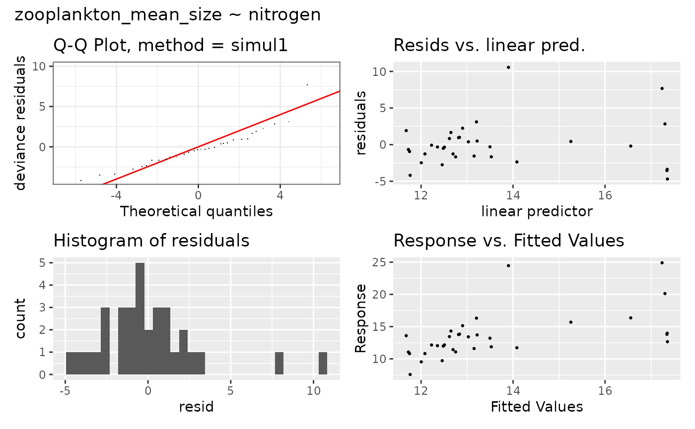
Let’s continue by calculating the vulnerability for both pathways
with the function vulnerability(). The vulnerability
function combines exposure, sensitivity and adaptive capacity into the
vulnerability score. For negative sensitivity score the following
function applies:
and for positive scores:
,
where V = vulnerability, S = sensitivity, AC = adaptive capacity and
E = exposure. For trait based scoring this will be done for each trait
individually. The vulnerabilities of each trait will then be aggregated;
we can decide with the parameter method_v if we want to use
an arithmetic mean, median, minimum or maximum for the aggregation, same
applies for aggregation of trait based uncertainty scores.
vuln_experts <- vulnerability(
  exposure_results = exp_expert,
  sensitivity_results = sens_ac_expert,
  method_vulnerability = "mean",
  method_uncertainty = "mean"
)

vuln_model <- vulnerability(
  exposure_results = exposure_model,
  sensitivity_results = sens_ac_model,
  method_vulnerability = "mean",
  method_uncertainty = "mean"
)

head(vuln_experts)
#>       indicator    pressure            type pathway vulnerability uncertainty
#> 1 phytoplankton temperature          direct  expert         -4.75    1.333333
#> 2 phytoplankton    salinity          direct  expert          0.00    2.000000
#> 3 phytoplankton      oxygen          direct  expert         -2.25    2.166667
#> 4 phytoplankton    nutrient          direct  expert         -4.25    2.000000
#> 5 phytoplankton     fishing          direct  expert          0.00    1.250000
#> 6 phytoplankton temperature direct_indirect  expert         -5.75    1.333333
head(vuln_model)
#>               indicator      pressure            type pathway vulnerability
#> 1 zooplankton_mean_size      nitrogen direct_indirect   model          6.25
#> 2 zooplankton_mean_size   phosphorous direct_indirect   model          0.00
#> 3 zooplankton_mean_size surf_temp_sum direct_indirect   model          0.00
#> 4 zooplankton_mean_size  bot_temp_ann direct_indirect   model          0.00
#> 5 zooplankton_mean_size  surf_sal_sum direct_indirect   model          4.25
#> 6 zooplankton_mean_size   bot_sal_ann direct_indirect   model          3.75
#>   uncertainty
#> 1         2.0
#> 2         1.5
#> 3         1.5
#> 4         1.5
#> 5         2.0
#> 6         2.5
The output of the vulnerability gives us for each indicator pressure type combination the vulnerability score with its associated uncertainty and the pathway with which the vulnerability has been determined.
To calculate the risk we need to know whether the indicator is currently in a good or undesired state, since the risk to be in an undesired state is higher if the indicator is already in it. Status can be determined by the experts or using the time series of the indicator. Our experts have assessed that phytoplankton and seabirds are currently in a good state, but herring and cod unfortunately not. An undesired state gets a score of −1 and a good state of +1.
status_experts <- data.frame(
  indicator = c("phytoplankton", "herring", "cod", "seabirds"),
  status = c("good", "undesired", "undesired", "good"),
  score = c(1, -1, -1, 1)
)
status_experts
#>       indicator    status score
#> 1 phytoplankton      good     1
#> 2       herring undesired    -1
#> 3           cod undesired    -1
#> 4      seabirds      good     1
In the modelling pathway the function status() evaluates
indicator status based on time series. To assess the status we have to
set baseline conditions where the indicator is assumed to be in a good
status and our assessment time frame for which the status shall be
evaluated (similar to the model_exposure() function).
Additionally we can set a range around the baseline mean which is
considered as good status. We can specify whether it is undesired if the
indicator is in the assessment time period below or above this range
using the arguments sign and condition. For
our status assessment we assume good baseline conditions in the first
ten years as the mean ± 1 standard deviation. Undesired status is
defined as being below 1 standard deviation so we set
sign = "-" and condition = "<".
status_model <- status(
  indicator_time_series = ts_indicators,
  base_years = c(start = 1984, end = 1993),
  current_years = c(start = 2012, end = 2016),
  sign = "-",
  condition = "<"
)
status_model
#>               indicator    status score
#> 1 zooplankton_mean_size undesired    -1
#> 2    eastern_baltic_cod undesired    -1
Both of our indicators are in the assessment time period in an undesired status.
Now we combine vulnerability and status to the final risk scores.
Both pathways use the function risk().
risk_expert <- risk(
  vulnerability = vuln_experts,
  status = status_experts
)
risk_model <- risk(
  vulnerability = vuln_model,
  status = status_model
)

head(risk_expert)
#>       indicator    pressure            type pathway vulnerability status  risk
#> 1 phytoplankton temperature          direct  expert         -4.75   good -3.75
#> 2 phytoplankton    salinity          direct  expert          0.00   good  0.00
#> 3 phytoplankton      oxygen          direct  expert         -2.25   good -1.25
#> 4 phytoplankton    nutrient          direct  expert         -4.25   good -3.25
#> 5 phytoplankton     fishing          direct  expert          0.00   good  0.00
#> 6 phytoplankton temperature direct_indirect  expert         -5.75   good -4.75
#>   uncertainty
#> 1    1.333333
#> 2    2.000000
#> 3    2.166667
#> 4    2.000000
#> 5    1.250000
#> 6    1.333333
head(risk_model)
#>               indicator      pressure            type pathway vulnerability
#> 1 zooplankton_mean_size      nitrogen direct_indirect   model          6.25
#> 2 zooplankton_mean_size   phosphorous direct_indirect   model          0.00
#> 3 zooplankton_mean_size surf_temp_sum direct_indirect   model          0.00
#> 4 zooplankton_mean_size  bot_temp_ann direct_indirect   model          0.00
#> 5 zooplankton_mean_size  surf_sal_sum direct_indirect   model          4.25
#> 6 zooplankton_mean_size   bot_sal_ann direct_indirect   model          3.75
#>      status risk uncertainty
#> 1 undesired 5.25         2.0
#> 2 undesired 0.00         1.5
#> 3 undesired 0.00         1.5
#> 4 undesired 0.00         1.5
#> 5 undesired 3.25         2.0
#> 6 undesired 2.75         2.5
The output of the risk function gives us per indicator–pressure–type combination the risk, calculated from vulnerability and status, as well as the uncertainty associated with the risk evaluation. Before we combine both data frames we will rename the pressure variables of the model based risk assessment to align with the names of the expert based assessment. This is necessary to correctly aggregate the risk values per pressure to multi pressure risk scores. Furthermore we will select for each pressure, which has more than one variable, one of them. We follow here a precautionary approach, thus we will select the one posing the highest risk.
risk_model <- risk_model[c(1, 3, 5, 7, 8, 9, 12, 14:16), ]
risk_model$pressure <- c(
  "nutrient", "temperature", "salinity", "oxygen", "fishing",   # for zooplankton
  "nutrient", "temperature", "salinity", "oxygen", "fishing")   # for cod
Now we combine both risk assessment data sets and aggregate them to get multi pressure, multi indicator and ecosystem risk scores. The aggregated score will automatically be calculated per pathway, type, pathway and type, and without accounting for type or pathway.
risks <- rbind(risk_expert, risk_model)

aggregated_risk <- aggregate_risk(
  risk_results = risks,
  method = "mean"
)

aggregated_risk$multi_indicator_risk
#>       pressure            type  pathway      risk uncertainty
#> 5      fishing          direct   expert -5.062500    1.416667
#> 10     fishing direct_indirect   expert -6.250000    1.416667
#> 15     fishing direct_indirect    model  1.625000    2.500000
#> 20     fishing          direct combined -5.062500    1.416667
#> 25     fishing direct_indirect combined -3.625000    1.777778
#> 30     fishing        combined   expert -5.656250    1.416667
#> 35     fishing        combined    model  1.625000    2.500000
#> 40     fishing        combined combined -4.200000    1.633333
#> 4     nutrient          direct   expert -1.250000    2.083333
#> 9     nutrient direct_indirect   expert -2.140625    2.083333
#> 11    nutrient direct_indirect    model  0.000000    2.000000
#> 19    nutrient          direct combined -1.250000    2.083333
#> 24    nutrient direct_indirect combined -1.427083    2.055556
#> 29    nutrient        combined   expert -1.695312    2.083333
#> 31    nutrient        combined    model  0.000000    2.000000
#> 39    nutrient        combined combined -1.356250    2.066667
#> 3       oxygen          direct   expert -2.468750    2.250000
#> 8       oxygen direct_indirect   expert -4.187500    2.250000
#> 14      oxygen direct_indirect    model -2.500000    1.500000
#> 18      oxygen          direct combined -2.468750    2.250000
#> 23      oxygen direct_indirect combined -3.625000    2.000000
#> 28      oxygen        combined   expert -3.328125    2.250000
#> 34      oxygen        combined    model -2.500000    1.500000
#> 38      oxygen        combined combined -3.162500    2.100000
#> 2     salinity          direct   expert -1.812500    1.750000
#> 7     salinity direct_indirect   expert -3.734375    1.750000
#> 13    salinity direct_indirect    model  1.625000    2.250000
#> 17    salinity          direct combined -1.812500    1.750000
#> 22    salinity direct_indirect combined -1.947917    1.916667
#> 27    salinity        combined   expert -2.773438    1.750000
#> 33    salinity        combined    model  1.625000    2.250000
#> 37    salinity        combined combined -1.893750    1.850000
#> 1  temperature          direct   expert -4.281250    1.416667
#> 6  temperature direct_indirect   expert -6.750000    1.416667
#> 12 temperature direct_indirect    model -3.750000    1.500000
#> 16 temperature          direct combined -4.281250    1.416667
#> 21 temperature direct_indirect combined -5.750000    1.444444
#> 26 temperature        combined   expert -5.515625    1.416667
#> 32 temperature        combined    model -3.750000    1.500000
#> 36 temperature        combined combined -5.162500    1.433333
aggregated_risk$multi_pressure_risk
#>                indicator            type  pathway     risk uncertainty
#> 3                    cod          direct   expert -5.03750    1.616667
#> 7                    cod direct_indirect   expert -7.20000    1.616667
#> 13                   cod          direct combined -5.03750    1.616667
#> 17                   cod direct_indirect combined -7.20000    1.616667
#> 23                   cod        combined   expert -6.11875    1.616667
#> 29                   cod        combined combined -6.11875    1.616667
#> 10    eastern_baltic_cod direct_indirect    model -2.90000    2.000000
#> 20    eastern_baltic_cod direct_indirect combined -2.90000    2.000000
#> 26    eastern_baltic_cod        combined    model -2.90000    2.000000
#> 32    eastern_baltic_cod        combined combined -2.90000    2.000000
#> 2                herring          direct   expert -3.26250    1.616667
#> 6                herring direct_indirect   expert -4.50000    1.616667
#> 12               herring          direct combined -3.26250    1.616667
#> 16               herring direct_indirect combined -4.50000    1.616667
#> 22               herring        combined   expert -3.88125    1.616667
#> 28               herring        combined combined -3.88125    1.616667
#> 1          phytoplankton          direct   expert -1.65000    1.750000
#> 5          phytoplankton direct_indirect   expert -2.25000    1.750000
#> 11         phytoplankton          direct combined -1.65000    1.750000
#> 15         phytoplankton direct_indirect combined -2.25000    1.750000
#> 21         phytoplankton        combined   expert -1.95000    1.750000
#> 27         phytoplankton        combined combined -1.95000    1.750000
#> 4               seabirds          direct   expert -1.95000    2.150000
#> 8               seabirds direct_indirect   expert -4.50000    2.150000
#> 14              seabirds          direct combined -1.95000    2.150000
#> 18              seabirds direct_indirect combined -4.50000    2.150000
#> 24              seabirds        combined   expert -3.22500    2.150000
#> 30              seabirds        combined combined -3.22500    2.150000
#> 9  zooplankton_mean_size direct_indirect    model  1.70000    1.900000
#> 19 zooplankton_mean_size direct_indirect combined  1.70000    1.900000
#> 25 zooplankton_mean_size        combined    model  1.70000    1.900000
#> 31 zooplankton_mean_size        combined combined  1.70000    1.900000
The aggregated risk scores are in three lists:
One with all risks aggregated per pressure,
one aggregated per indicator and
one with the ecosystem risk, which is an aggregation of all multi pressure risk scores.
In all lists the scores are first aggregated per type and pathway, then per type regardless of the pathway, then per pathway regardless of the type and as last regardless of the type and pathway.
Results
To get an easier overview of the results and help with the
interpretation ecorisk provides two plotting functions
plot_radar() and plot_heatmap().
The first one creates for each indicator a radar plot with the risk scores per pressure and type. In the centre it shows the aggregated multi-pressure risk; we have to select which we want to use. This plot helps to identify per indicator the most influencing pressures and compare results from different types. If uncertainty has been assessed this will be displayed as a ring around the radar plot. In this example we will use the aggregated score of direct and indirect effects, regardless of the pathway. These are assumed to better reflect reality compared to direct effects only.
p_radar <- plot_radar(
  risk_scores = risks,
  aggregated_scores = aggregated_risk,
  type = "direct_indirect",
  pathway = "combined"
)

p_radar[[1]]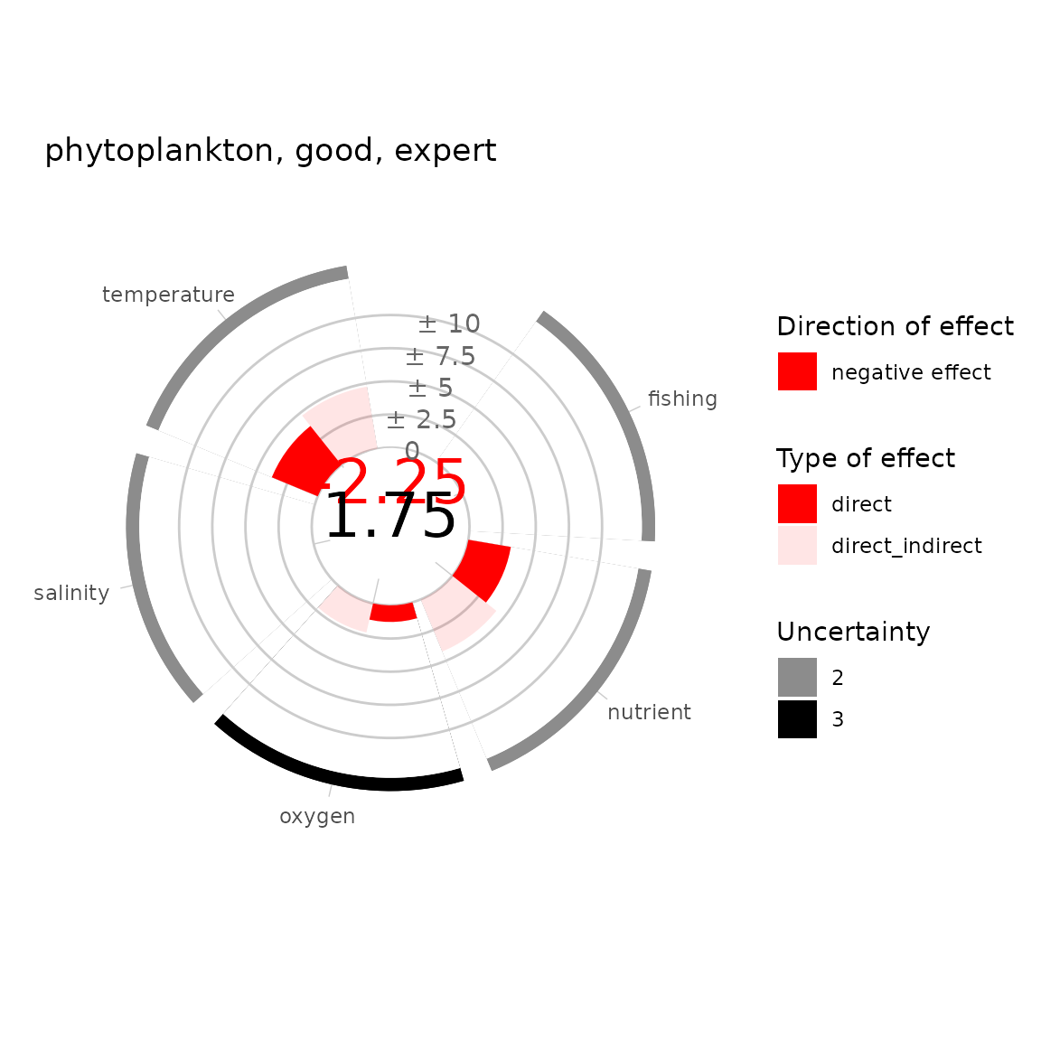
p_radar[[2]]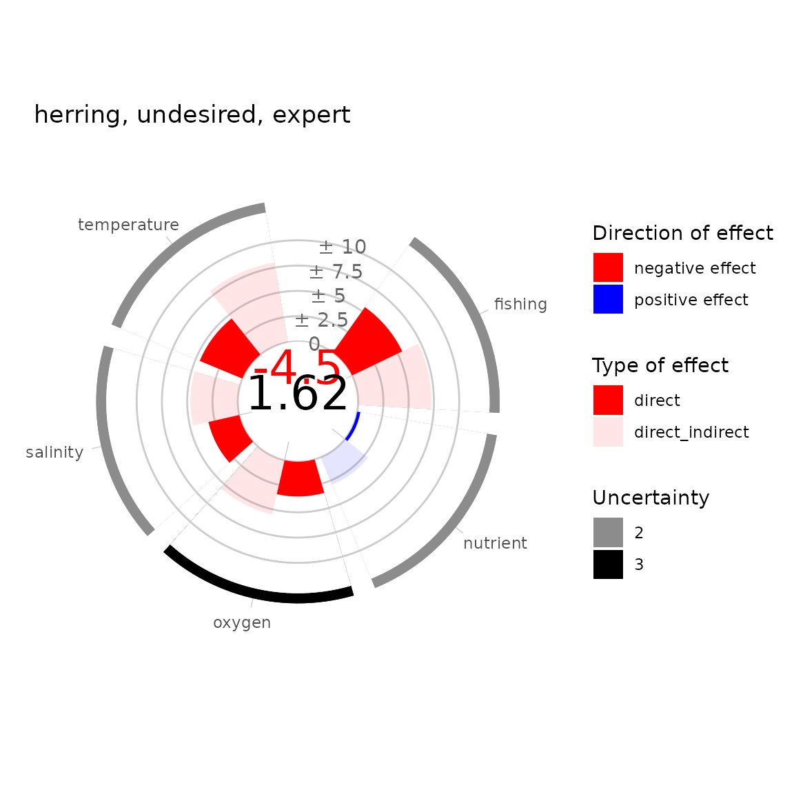
p_radar[[3]]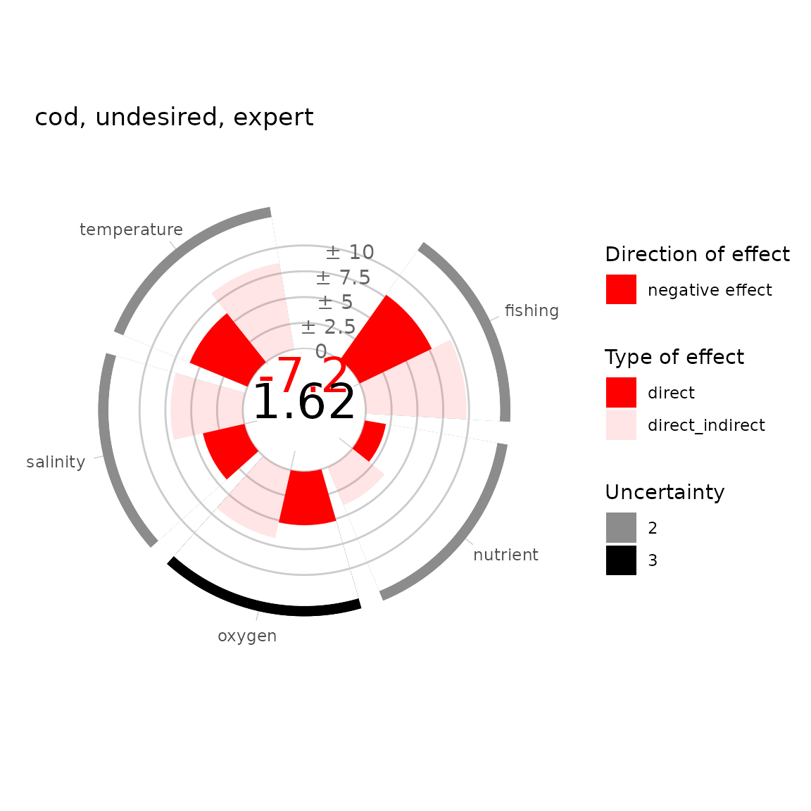
p_radar[[4]]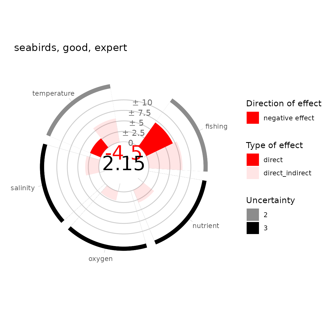
p_radar[[5]]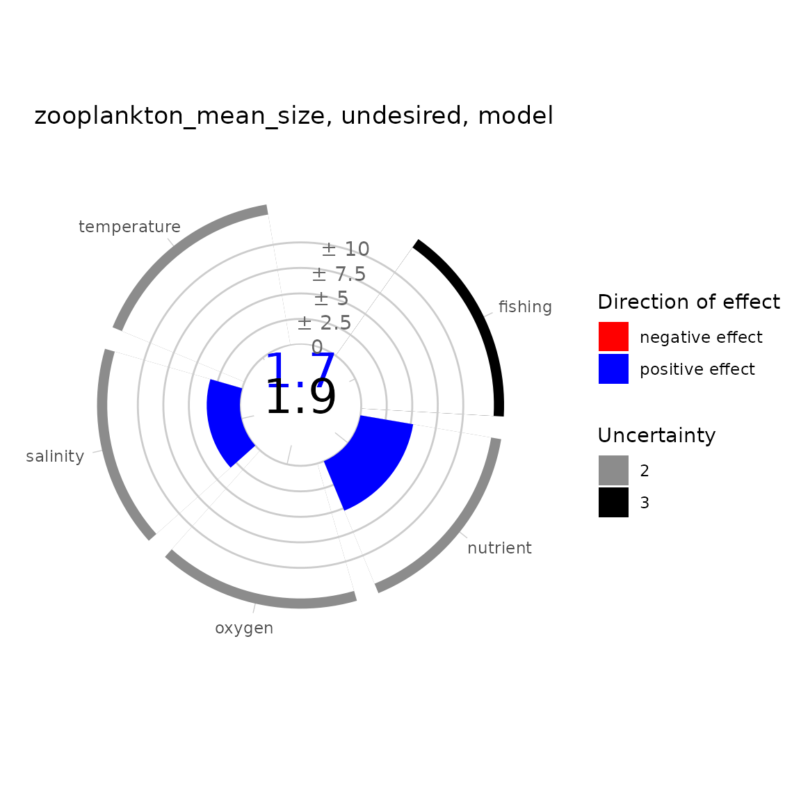
p_radar[[6]]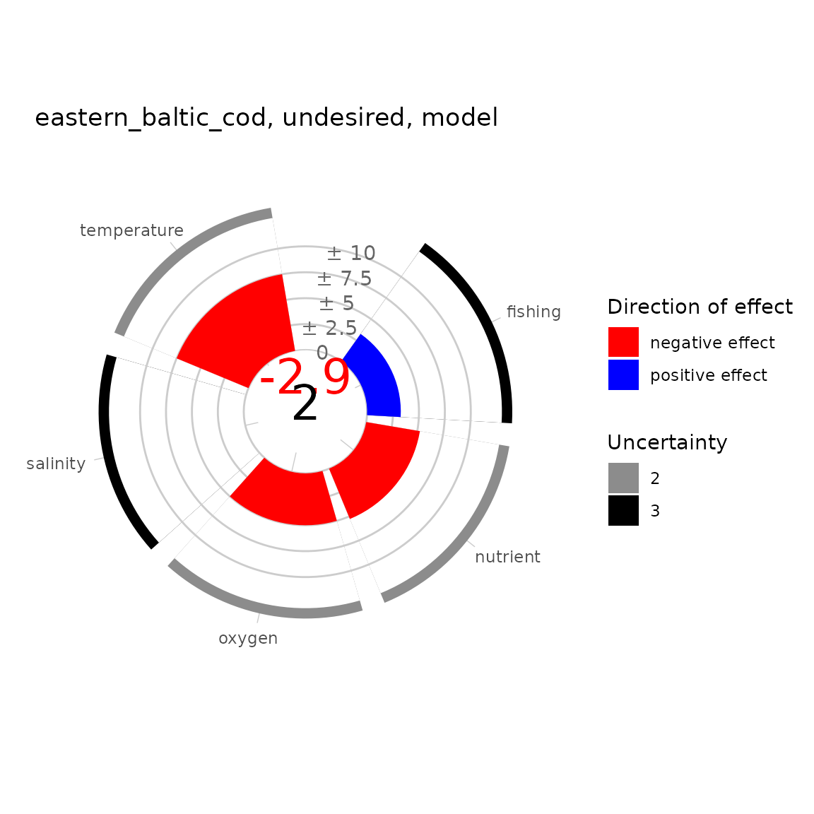
All of the indicators have a negative multi-pressure score. The indicators assessed with the expert scoring pathway show a higher risk due to the combined direct and indirect effects compared to direct effects only. The uncertainty is generally lower in the modelling pathway. Comparing the modelling and expert pathway for cod it is noticeable that both have a similar multi-pressure score but the individual risk scores are quite different: The experts assessed fishing as the most influencing pressure, whereas in the modelling pathway salinity is considered as the pressure with the highest impact. To directly compare modelling and expert pathway for cod we can correlate them in a plot:
temp <- risks[c(26:30, 45:49), c(1, 2, 7)]
temp <- temp |>
  tidyr::pivot_wider(names_from = indicator, values_from = risk)

ggplot2::ggplot(dat = temp,
    ggplot2::aes(x = cod, y = eastern_baltic_cod, colour = pressure)) +
  ggplot2::geom_point() +
  ggplot2::geom_abline(slope = 1, intercept = 0) +
  ggplot2::xlim(-10, 10) +
  ggplot2::ylim(-10,10) +
  ggplot2::labs(x = "Expert-based pathway", y = "Modelling-based pathway") +
  ggplot2::theme_minimal()
#> Warning: Removed 1 row containing missing values or values outside the scale range
#> (`geom_point()`).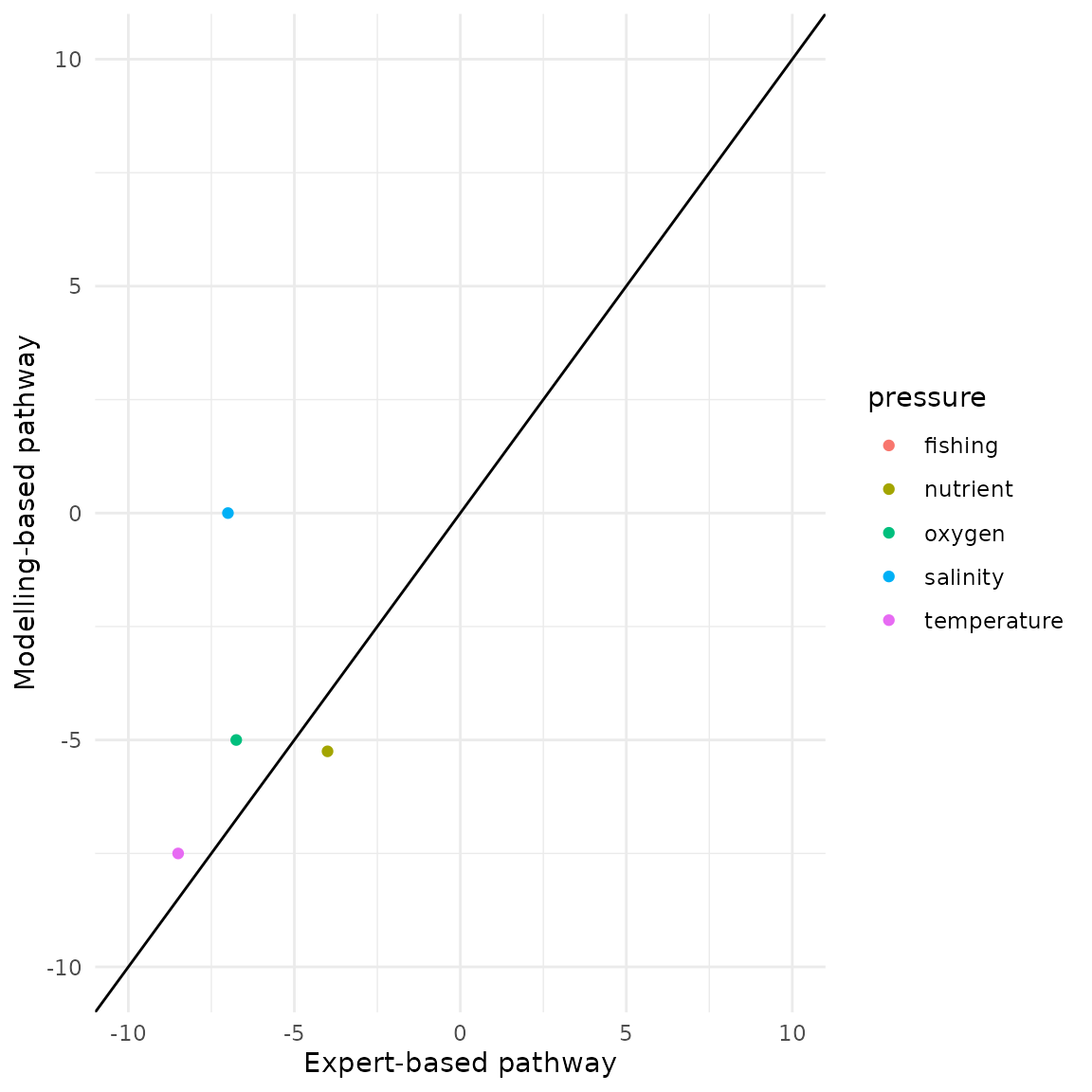
We can see that the risk scores for nutrients, oxygen and temperature
are quite similar for both pathways. But the values for salinity
indicate no risk in the modelling pathway. This might be due to a
salinity time series that does not catch the ongoing dynamics, and thus
resulting in a non-significant relationship between pressure and
indicator. The scores for fishing have even opposing directions; this
could be due to a different understanding of fishing and the future
developments: In the modelling pathway it has been shown that fishing is
decreasing, which will be positive for the indicators, thus in the
future it will have a positive effect. But the expert probably assumed
that fishing will always have negative effects, without considering the
positive development of the decreasing fishing pressure. This is a
linguistic uncertainty, which should have been discussed in the planning
and scoping phase of the assessment, to ensure that all have a common
understanding. Nevertheless we should reiterate with our experts as well
as check if the model_sensitivity() and
model_exposure() functions have correctly determined the
effect direction.
The function plot_heatmap() creates for each assessment
type a heatmap of all pressure indicator combinations, optionally with
the associated uncertainty. The aggregated multi-pressure and indicator
scores are shown at the bottom and to the left of the heatmap as well as
the system risk score at the bottom right. For the aggregated scores we
have to choose which one we want to use as we already did for the
plot_radar() function. This function gives a complete
overview of the system dynamics allowing to easily compare ecosystems
and determine by which indicators and pressures ecosystem risk is
driven.
p_heat <- plot_heatmap(
  risk_scores = risks,
  aggregated_scores = aggregated_risk,
  uncertainty = TRUE
)
#> Registered S3 method overwritten by 'car':
#>   method           from
#>   na.action.merMod lme4

p_heat[[1]]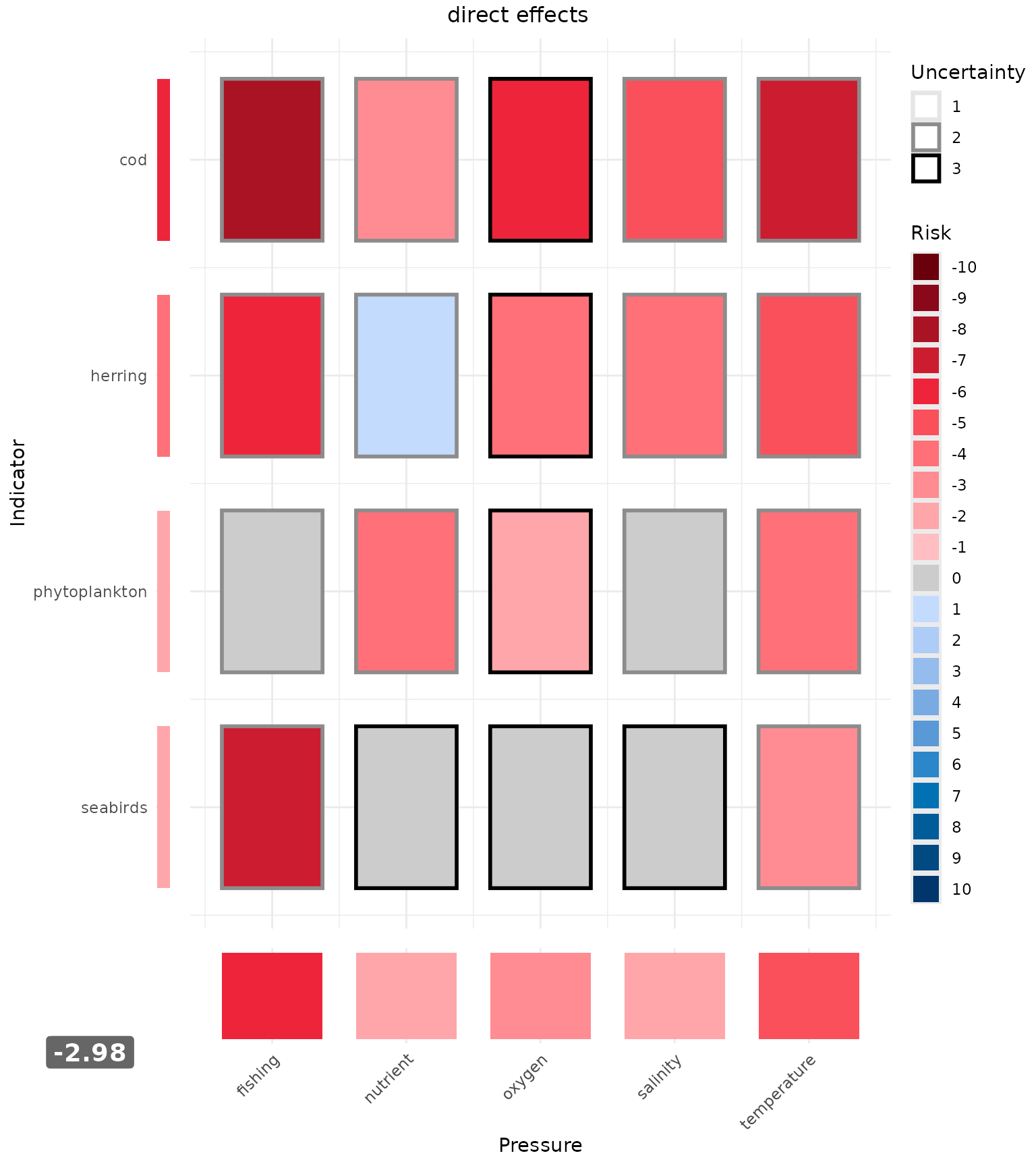
p_heat[[2]]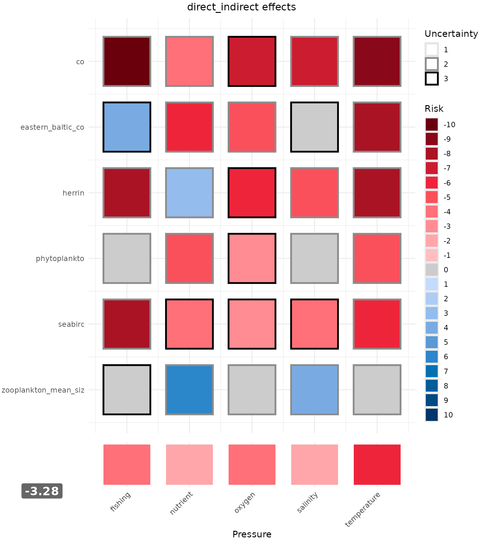
The first heatmap includes only direct effects, thus this heatmap is a bit smaller as we did not assess for all indicators direct effects only. The multi pressure and indicator scores are the aggregated direct scores for all assessed pathways. The grey frame around the heatmap tiles show the uncertainty associated with the score. We can see with this heatmap that cod is the indicator most at risk, this risk is due to high effects of fishing and temperature. The least at risk indicators are phytoplankton and seabirds. Both are not affected by several of the pressures, but still seabirds are at a medium to high risk due to fishing. The second heatmap shows the direct and indirect effects including also the indicator which were assessed with the modelling pathway. Again the cod indicator is most at risk, followed by the modelled cod indicator, herring and seabirds. The pressures with the highest negative impact are temperature and fishing. Zooplankton is an example for an indicator which will likely thrive under the pressures. It is still worthwhile to include such indicators in a risk assessment as these positive changes in one indicator can have negative effects for the entire system, thus every change can bear a risk for the system. Overall the system is a bit more at risk considering the combination of direct and indirect effects compared to direct effects only.
What can we do now with the results of our risk assessment? Here are some examples:
- We can inform the management by prioritizing which pressures pose the highest risk and which indicators are most at risk.
- We can use the information to guide research: did any effect come by surprise (especially from the modelling pathway)? Which risks are associated with high uncertainties?
- If we are interested in non-linear effects and how indicators and pressures interact with each other we could use our results as a basis for a network analysis and develop questions based on the risk assessment output or select specific indicator and pressure combinations that we want to further investigate with a more quantitative analysis.
Contact
If you have issues with the package or questions please send an e-mail to: helene.gutte@uni-hamburg.de